Comparing hyperparameter tuning strategies with tidymodels

Photo by Jonathan Farber

tl;dr

We compare 5 hyperparameter tuning search strategies in terms of (a) model quality and (b) run time on 10 learning problems with 3 machine learning algorithms using the tidymodels framework. Bayesian search gave best results, while the racing methods had lowest running time. When interpreting the results, it must be taken into account that the search strategies have their own hyperparameters, which can substantially influence the results.

Introduction

Hyperparameter tuning is a crucial step in building machine learning (ML) models. Hyperparameters influence the learning process of ML algorithms, thus they are a decisive factor for model performance. A challenge is that generally, the optimal hyperparameter setting cannot be derived directly from the data before model training. A popular tuning approach is grid search, which involves first defining sets of candidate hyperparameter values, then training a separate ML model for each setting and evaluating their performance on a holdout dataset to finally select the setting with the best performance.

Flexible models usually have more hyperparameters which requires evaluating large tuning grids. For instance, gradient boosted trees are considered as state-of-the-art models for non-perceptual (tabular) data, but they involve many hyperparameters, e.g. the number of predictors randomly sampled at each base tree split, the number of trees in the ensemble, the minimum number of observations in a tree node for a further split to be attempted, the learning rate determining the weight of the last created tree towards the prediction of the ensemble, and more. A grid search for an ML algorithm with only 4 hyperparameters and 10 candidate values each requires evaluating 10^4^=10,000 models. Quiet a lot!

Iterative search methods are alternatives to this brute-force approach, as they pursue different search strategies that may be less computationally expensive as fewer evaluations are required. The basic idea of iterative search is to exploit the existing tuning results to decide which candidate hyperparameter setting to try next.

The tune package of the tidymodels ecosystem implements both grid search and the iterative Bayesian search. I recently stumbled upon the finetune package, which provides three more iterative search methods, simulated annealing, racing with ANOVA models, and racing with win/loss statistics.

This post describes a case study to explore the potential of iterative search by comparing four iterative search methods with grid search in terms of (a) predictive performance and (b) running time of the tuning process.

A glimpse of the basic ideas of the four iterative search methods are as follows:

• tune::tune_bayes(): In Bayesian tuning¹, the relationship between hyperparameter search space and model performance is captured in a probabilistic surrogate model, which is iteratively refined as more hyperaprameter value combinations are evaluated. An important aspect is the so-called acquisition function, which determines which candidate hyperparameter values to evaluate next. Acquisition functions often trade off exploration and exploitation. In terms of exploration, an area of the search space is promising if there is high uncertainty in the surrogate model (we don’t know how good the model will be), whereas exploitation favors areas of the search space with high model prediction accuracy (we know that similar hyperparameter settings lead to well-performing models).
• finetune::tune_sim_anneal(): At each iteration of simulated annealing^{2 3}, a new hyperparameter setting is created by randomly perturbing the current hyperparameter setting slightly. If the model performance of this new setting outperforms the current setting, we accept the new setting. If the new setting is inferior to the current one, we do not always reject it, but decide based on an acceptance probability threshold whether to keep it. This element of randomness allows simulated annealing to bypass local optima.
• Racing methods⁴: In their so-called burn in phase, all hyperparameter candidate settings are evaluated on only a small set of resamples. Based on some criterion, hyperparameter candidate settings that are unlikely to be the best at the end are removed and the remaining settings are evaluated on the next resample. The process continues until there is only one hyperparameter candidate setting left or the maximum number of resamples is reached.
  • finetune::tune_race_anova(): The criterion to filter out hyperparameter candidate settings without prospect of success is based on a repeated measures ANOVA model.
  • finetune::tune_race_win_loss(): A Bradley-Terry model estimates the likelihood of a hyperparameter setting to be the overall winner. A candidate setting is dropped if its confidence interval indicates futility w.r.t. the remaining resamples.

Setup

First, we load all required packages.

suppressPackageStartupMessages({
  library(tidyverse)
  library(tidymodels)
  library(finetune)
  library(ranger)
  library(kernlab)
  library(xgboost)
})

For our comparison, we use ten datasets from the modeldata package, eight of which have a binominal target and two have a numeric target. We create a data frame in which each row represents a dataset, where target is the name of the target variable, and positive is the value of the positive class. Datasets with a numeric target variable have an NA value in positive.

datasets <- tribble(
            ~name,      ~target,  ~positive,
        "ad_data",      "Class", "Impaired",
           "ames", "Sale_Price",         NA,
      "attrition",  "Attrition",      "Yes",
     "car_prices",      "Price",         NA,
          "cells",      "class",       "PS",
    "credit_data",     "Status",      "bad",
   "lending_club",      "Class",      "bad",
      "mlc_churn",      "churn",      "yes",
  "stackoverflow",     "Remote",   "Remote",
       "wa_churn",      "churn",      "Yes"
  )

Next, we define the ML algorithm, their hyperparameters which we will tune, and we specify the tuning methods. We will use random forests (with 3 hyperparameters), gradient boosted trees (5), and polynominal support vector machines (4).

algorithms <- bind_rows(
  tibble(
    algorithm = "rand_forest",
    spec = list(rand_forest(mtry = tune(), trees = tune(), min_n = tune()) |> 
                  set_engine("ranger"))
  ),
  tibble(
    algorithm = "boost_tree",
    spec = list(boost_tree(mtry = tune(), trees = tune(), tree_depth = tune(), 
                           learn_rate = tune(), sample_size = tune()) |>
                  set_engine("xgboost"))
  ),
  tibble(
    algorithm = "svm_poly",
    spec = list(svm_poly(cost = tune(), degree = tune(), scale_factor = tune(),
                         margin = tune()) |>
                  set_engine("kernlab"))
  )
)

We create a data frame that contains the names of the tuning search strategies.

tuning <- tibble(
  tuning = c("grid", "bayes", "sim_anneal", "race_anova", "race_win_loss")
)

Next, we augment datasets with the following columns:

• data: the actual dataset. We set the target variable as the dataset’s first column. If it is a classification problem, we convert the target variable to a factor and set the positive class as first level.
• model: either "classification" or "regression"
• rep: iteration number. We repeat each evaluation process 5 times, using different training and test sets each time.
• train and test: the stratified training (70%) and test (30%) sets
• rs: the resampled training data. We use stratified 10-fold cross-validation here.

n_reps <- 5L
prop_tuning <- 0.7
n_folds <- 10L

set.seed(1)
datasets <- datasets |>
  # make the dataset available in the environment,
  # set the target variable as first column,
  # convert a binominal target variable to a factor and 
  # set the positive class as first level
  mutate(data = pmap(
    list(name, target, positive),
    function(name, target, positive) {
      data(list = name)
      df <- eval(sym(name)) |>
        rename_with(~"target", all_of(target)) |>
        relocate(target, .before = 1)
      
      if (is.factor(df$target)) {
        df <- df |> mutate(target = fct_relevel(target, positive))
      }
      df
    }
  )) |>
  # set the mode (classification vs. regression model)
  mutate(mode = map_chr(data, ~ {
    ifelse(is.factor(.x$target), "classification", "regression")
  })) |>
  # repeat each row n_reps times
  full_join(
    expand_grid(name = unique(datasets$name), rep = 1:n_reps),
    by = "name"
  ) |>
  # split the data into train and test set
  mutate(
    split = map(data, initial_split, prop = prop_tuning, strata = target)
  ) |>
  mutate(train = map(split, ~ training(.x))) |>
  mutate(test = map(split, ~ testing(.x))) |>
  # extract resamples from the train data 
  mutate(rs = map(train, vfold_cv, v = n_folds, strata = target)) |>
  select(-data, -split)
datasets |> head()

## # A tibble: 6 × 8
##   name    target     positive mode             rep train    test     rs        
##   <chr>   <chr>      <chr>    <chr>          <int> <list>   <list>   <list>    
## 1 ad_data Class      Impaired classification     1 <tibble> <tibble> <vfold_cv>
## 2 ad_data Class      Impaired classification     2 <tibble> <tibble> <vfold_cv>
## 3 ad_data Class      Impaired classification     3 <tibble> <tibble> <vfold_cv>
## 4 ad_data Class      Impaired classification     4 <tibble> <tibble> <vfold_cv>
## 5 ad_data Class      Impaired classification     5 <tibble> <tibble> <vfold_cv>
## 6 ames    Sale_Price <NA>     regression         1 <tibble> <tibble> <vfold_cv>

We join data with algorithms and tuning, so that we get all combinations of dataset (10), repetition (5), algorithm (3), and tuning search method (5) (= 750 rows).

eval_grid <- datasets |>
  mutate(algorithms = list(algorithms), tuning = list(tuning)) |>
  unnest(cols = algorithms) |>
  unnest(cols = tuning) |>
  mutate(id = row_number(), .before = 1) |>
  mutate(id = str_pad(id, width = nchar(as.character(max(id))), pad = "0"))
eval_grid |> head()

## # A tibble: 6 × 12
##   id    name  target positive mode    rep train    test     rs         algorithm
##   <chr> <chr> <chr>  <chr>    <chr> <int> <list>   <list>   <list>     <chr>    
## 1 001   ad_d… Class  Impaired clas…     1 <tibble> <tibble> <vfold_cv> rand_for…
## 2 002   ad_d… Class  Impaired clas…     1 <tibble> <tibble> <vfold_cv> rand_for…
## 3 003   ad_d… Class  Impaired clas…     1 <tibble> <tibble> <vfold_cv> rand_for…
## 4 004   ad_d… Class  Impaired clas…     1 <tibble> <tibble> <vfold_cv> rand_for…
## 5 005   ad_d… Class  Impaired clas…     1 <tibble> <tibble> <vfold_cv> rand_for…
## 6 006   ad_d… Class  Impaired clas…     1 <tibble> <tibble> <vfold_cv> boost_tr…
## # … with 2 more variables: spec <list>, tuning <chr>

nrow(eval_grid)

## [1] 750

After that, we create a function my_tuning which performs the actual hyperparameter tuning and records the running time of the tuning process and the model performance.

First, we create a preprocessing recipe with the following steps:

1. set target as outcome
2. get rid of of missing values by mean imputation for numeric columns and mode imputation for factor columns
3. create dummy columns for factors with more than two levels.

Steps 2. and 3. are necessary as ML algorithms usually require complete and all-numeric data. If we really wanted to put the models into practice, we should think about smarter imputation strategies like MICE.

Then, we update the model specification with the correct mode, i.e., classification or regression. We combine the recipe and the model specification into a workflow object. As primary performance metric, we set AUROC for classification models and RMSE for regression models.

Next, perform hyperparameter tuning and record the elapsed time. Note that we do not specify candidate hyperparameter values ourselves, but leave it to tidymodels to populate a space-filling parameter grid. We also leave all the hyperparameters of the tuning search methods at their default values.

Using the optimal model hyperparameters, we fit a final model on the whole training set and compute its performance on the holdout set.

We return a list with two elements: the elapsed time and the final model’s test set performance.

my_tuning <- function(spec, tuning, rs, mode, train, test, verbose = FALSE) {
  
  rec <- recipe(target ~ ., data = train) |>
    update_role(target, new_role = "outcome") |>
    step_impute_mean(all_numeric(), - all_outcomes()) |>
    step_impute_mode(all_nominal(), - all_outcomes()) |>
    step_dummy(all_nominal(), -all_outcomes())
  
  spec <- spec |> set_mode(mode)
  
  wf <- workflow() |> 
    add_recipe(rec) |>
    add_model(spec)
  
  metric <- metric_set(roc_auc)
  if(mode != "classification") metric <- metric_set(rmse)
  
  start <- Sys.time()
  
  if(tuning == "grid") {
    res <- wf |> tune_grid(
      resamples = rs, 
      metrics = metric,
      grid = 10L,
      control = control_grid(verbose = verbose)
    )
  }
  
  if(tuning == "grid20") {
    res <- wf |> tune_grid(
      resamples = rs, 
      metrics = metric,
      grid = 20L,
      control = control_grid(verbose = verbose)
    )
  }
  
  if(tuning == "bayes") {
    res <- wf |> tune_bayes(
      resamples = rs, 
      metrics = metric,
      control = control_bayes(verbose = verbose),
      param_info = spec |> extract_parameter_set_dials() |> finalize(train)
    )
  }
  
  if(tuning == "sim_anneal") {
    res <- wf |> tune_sim_anneal(
      resamples = rs, 
      metrics = metric,
      control = control_sim_anneal(verbose = verbose),
      param_info = spec |> extract_parameter_set_dials() |> finalize(train)
    )
  }
  
  if(tuning == "race_anova") {
    res <- wf |> tune_race_anova(
      resamples = rs, 
      metrics = metric,
      control = control_race(verbose = verbose, verbose_elim = verbose),
      param_info = spec |> extract_parameter_set_dials() |> finalize(train)
    )
  }
  
  if(tuning == "race_win_loss") {
    res <- wf |> tune_race_win_loss(
      resamples = rs, 
      metrics = metric,
      control = control_race(verbose = verbose, verbose_elim = verbose),
      param_info = spec |> extract_parameter_set_dials() |> finalize(train)
    )
  }
  
  end <- Sys.time()
  
  final_model <- wf |> 
    finalize_workflow(select_best(res)) |>
    fit(train)
  
  if(mode == "classification") {
    test_perf <- final_model |>
      predict(test, type = "prob") |>
      select(.pred = 1) |>
      mutate(.truth = test$target) |>
      roc_auc(truth = .truth, estimate = .pred)
  } else {
    test_perf <- final_model |>
      predict(test) |>
      select(.pred = 1) |>
      mutate(.truth = test$target) |>
      rmse(truth = .truth, estimate = .pred)
  }
  
  list(
    time_elapsed = end - start,
    test_perf = test_perf
  )
}

Finally, we iterate my_tuning over eval_grid, e.g. using pmap()

eval_grid <- eval_grid |>
  mutate(tune_res = pmap(list(spec, tuning, rs, mode, train, test), my_tuning))

Results

We rank the tuning methods, for each combination of dataset (10), repetition (5), and algorithm (3), giving 250 ranks per tuning method. Since there are 5 tuning methods in total, the rank is between 1 and 5.

eval_grid <- read_rds("eval_grid.rds") |>
  mutate(algorithm = factor(
    algorithm,
    levels = c("rand_forest", "boost_tree", "svm_poly")
  )) |>
  mutate(
    tuning = factor(
      tuning,
      levels = c("grid", "bayes", "sim_anneal", "race_anova", "race_win_loss")
    )
  ) |>
  group_by(name, rep, algorithm) |>
  mutate(perf_best = 
           ifelse(.metric == "roc_auc", 
                  max(.estimate),
                  min(.estimate)
           )
  ) |>
  mutate(perf_rnk = 
           ifelse(.metric == "roc_auc", 
                  min_rank(-.estimate),
                  min_rank(.estimate)
           )
  ) |>
group_by(name, algorithm, rep) |>
  mutate(perf_rel = ifelse(.metric == "roc_auc", 
                      .estimate / perf_best,
                      1 - (.estimate - perf_best) / perf_best
  )) |>
  ungroup()
eval_grid 

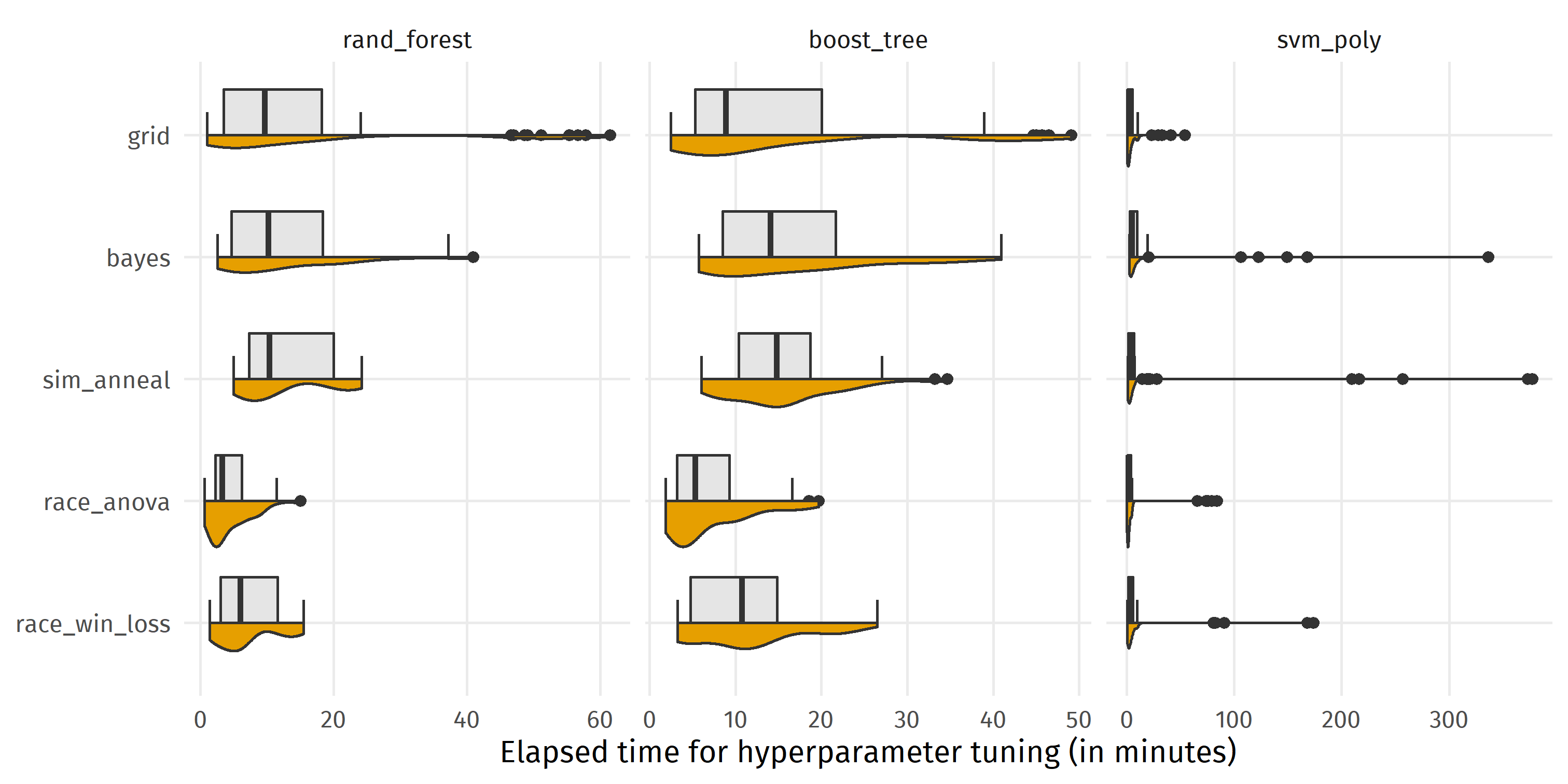
Comparing median running times in the figure below, we see that racing with ANOVA (race_anova) was fastest for random_forest (median = 3.3 min), boost_tree (5.3 min), and svm_poly (1.6 min). Regarding all 10 datasets x 5 repetitions * 3 algorithms = 150 pairwise comparisons of tuning methods, race_anova was faster than bayes 99.4% of the time and faster than sim_anneal 99.3% of the time, but none of the search strategies dominated one of the other search strategies for all runs. Having a closer look at the distributions reveals that although grid search was faster than bayes and sim_anneal, there were several settings with high running times for rand_forest and boost_tree (>40 min). Overall, grid was somewhat in the middle, winning against each of bayes, sim_anneal and race_win_loss for more than half of the comparisons.

ggplot(eval_grid, aes(y = time_elapsed / 60, x = fct_rev(tuning))) +
  coord_flip() +
  gghalves::geom_half_boxplot(side = "r", fill = "gray90") +
  gghalves::geom_half_violin(side = "l", fill = colorblindr::palette_OkabeIto[1]) +
  facet_wrap(~ algorithm, scales = "free_x") +
  labs(x = NULL, y = "Elapsed time for hyperparameter tuning (in minutes)")

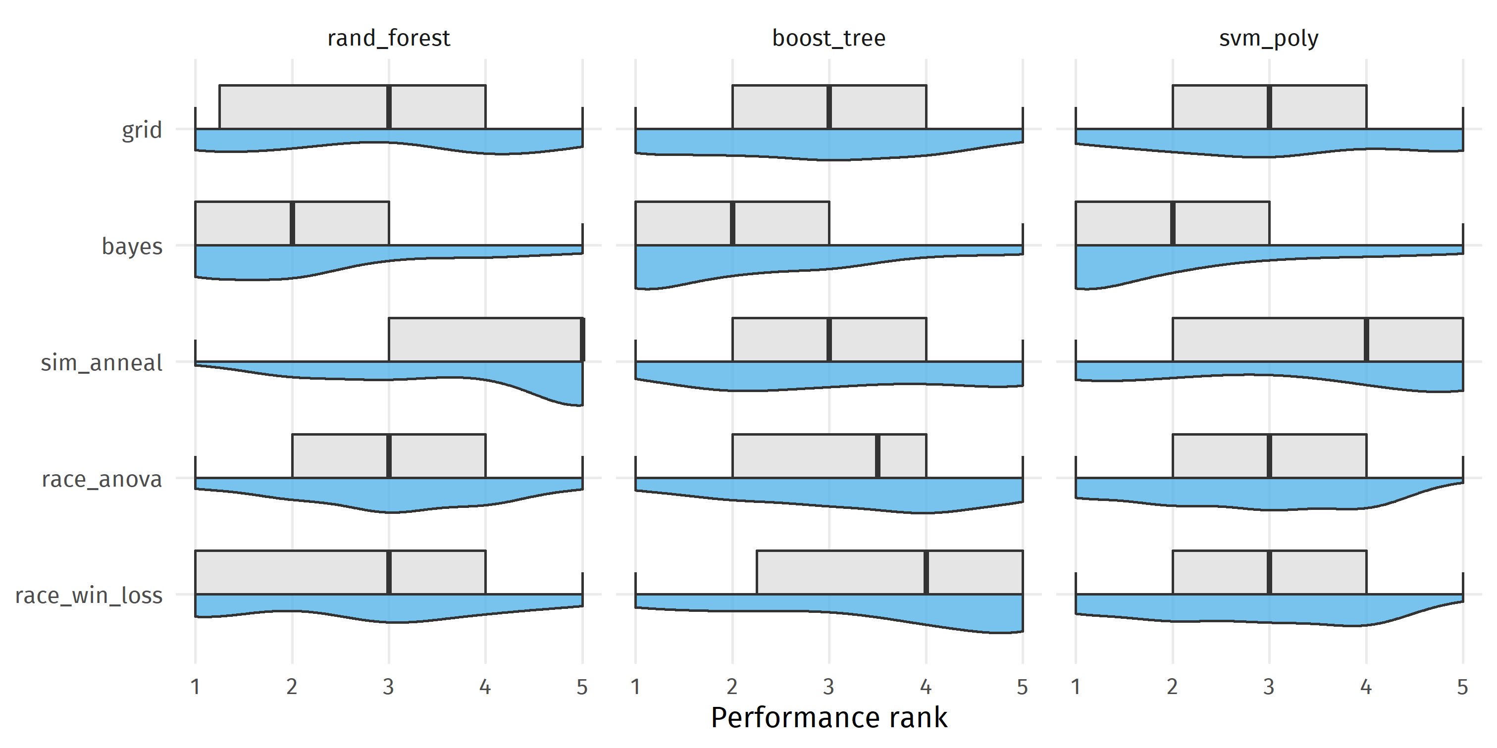
Comparing median performance ranks in the figure below, we see that bayes achieved the best result with a median rank of 2 for each modeling algorithm, whereas grid was ranked 3rd for each model algorithm. bayes was better than sim_anneal in 63.9% runs, better than race_win_loss in 60.0% of the runs, better than race_anova in 58.9% of the runs, and better than grid in 58.2% of the runs.

ggplot(eval_grid, aes(y = perf_rnk, x = fct_rev(tuning))) +
  coord_flip() +
  gghalves::geom_half_violin(side = "l", fill = colorblindr::palette_OkabeIto[2], 
                             alpha = 0.8) +
  gghalves::geom_half_boxplot(side = "r", fill = "gray90") +
  facet_wrap(~ algorithm, scales = "free_x") +
  labs(x = NULL, y = "Performance rank")

Discussion points

All tuning methods have their own hyperparameters which may influence both running time and predictive performance. For example, the racing methods have a burn_in parameter, with a default value of 3, meaning that all grid combinations must be run on 3 resamples before filtering of the parameters begins. Increasing this value can prevent early removal of seemingly futile but ultimately winning hyperparameters, but also results in higher run times. In this case study, we left it at the default settings.

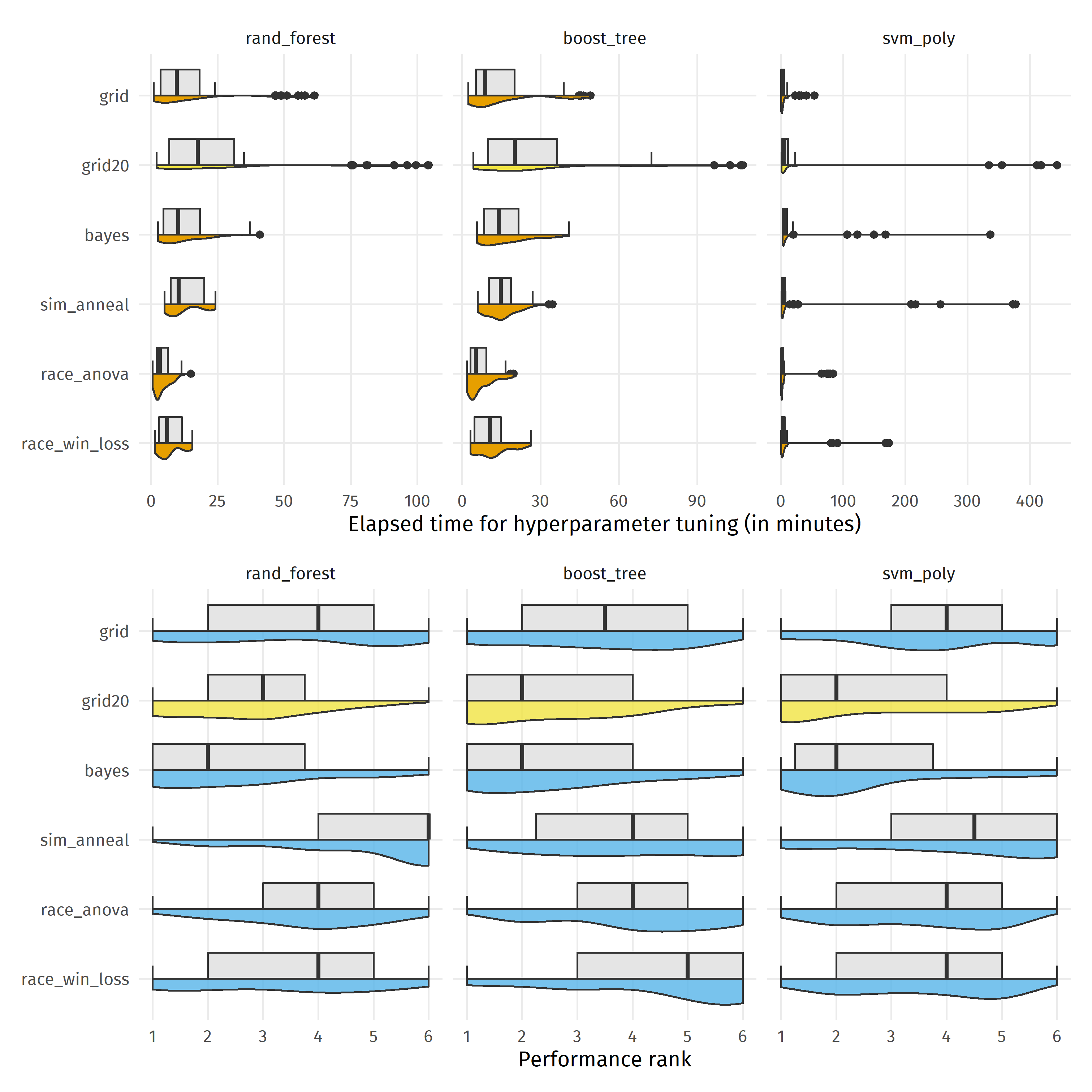
By default, tune_grid() uses only 10 candidate hyperparameter settings. In practice, we would rather use larger grids, especially if we have many hyperparameters to tune. However, if we just double the number of candidate settings to 20 (“grid20” in the plot below), grid search becomes the slowest (considering the median elapsed time) tuning method, but also very close in performance to the winning strategy bayes.

sessionInfo()

## R version 4.2.0 (2022-04-22 ucrt)
## Platform: x86_64-w64-mingw32/x64 (64-bit)
## Running under: Windows 10 x64 (build 22000)
## 
## Matrix products: default
## 
## locale:
## [1] LC_COLLATE=German_Germany.utf8  LC_CTYPE=German_Germany.utf8   
## [3] LC_MONETARY=German_Germany.utf8 LC_NUMERIC=C                   
## [5] LC_TIME=German_Germany.utf8    
## 
## attached base packages:
## [1] stats     graphics  grDevices utils     datasets  methods   base     
## 
## other attached packages:
##  [1] xgboost_1.6.0.1      kernlab_0.9-30       ranger_0.13.1       
##  [4] finetune_0.2.0       yardstick_0.0.9.9000 workflowsets_0.2.1  
##  [7] workflows_0.2.6.9001 tune_0.2.0.9001      rsample_0.1.1       
## [10] recipes_0.2.0        parsnip_0.2.1.9002   modeldata_0.1.1     
## [13] infer_1.0.0          dials_0.1.1          scales_1.2.0        
## [16] broom_0.8.0          tidymodels_0.2.0     forcats_0.5.1       
## [19] stringr_1.4.0        dplyr_1.0.9          purrr_0.3.4         
## [22] readr_2.1.2          tidyr_1.2.0          tibble_3.1.7        
## [25] ggplot2_3.3.6        tidyverse_1.3.1     
## 
## loaded via a namespace (and not attached):
##  [1] colorspace_2.0-3   ellipsis_0.3.2     class_7.3-20       fs_1.5.2          
##  [5] rstudioapi_0.13    farver_2.1.0       listenv_0.8.0      furrr_0.3.0       
##  [9] prodlim_2019.11.13 fansi_1.0.3        lubridate_1.8.0    xml2_1.3.3        
## [13] codetools_0.2-18   splines_4.2.0      extrafont_0.18     knitr_1.39        
## [17] jsonlite_1.8.0     colorblindr_0.1.0  Rttf2pt1_1.3.10    dbplyr_2.1.1      
## [21] compiler_4.2.0     httr_1.4.3         backports_1.4.1    assertthat_0.2.1  
## [25] Matrix_1.4-1       fastmap_1.1.0      cli_3.3.0          htmltools_0.5.2   
## [29] tools_4.2.0        gtable_0.3.0       glue_1.6.2         Rcpp_1.0.8.3      
## [33] cellranger_1.1.0   jquerylib_0.1.4    DiceDesign_1.9     vctrs_0.4.1       
## [37] blogdown_1.10      extrafontdb_1.0    gghalves_0.1.3     iterators_1.0.14  
## [41] timeDate_3043.102  gower_1.0.0        xfun_0.31          globals_0.15.0    
## [45] rvest_1.0.2        lifecycle_1.0.1    future_1.26.1      MASS_7.3-56       
## [49] ipred_0.9-12       hms_1.1.1          parallel_4.2.0     yaml_2.3.5        
## [53] sass_0.4.1         rpart_4.1.16       stringi_1.7.6      highr_0.9         
## [57] foreach_1.5.2      lhs_1.1.5          hardhat_1.0.0      lava_1.6.10       
## [61] rlang_1.0.2        pkgconfig_2.0.3    evaluate_0.15      lattice_0.20-45   
## [65] patchwork_1.1.1    labeling_0.4.2     tidyselect_1.1.2   parallelly_1.31.1 
## [69] magrittr_2.0.3     bookdown_0.26      R6_2.5.1           generics_0.1.2    
## [73] DBI_1.1.2          pillar_1.7.0       haven_2.5.0        withr_2.5.0       
## [77] survival_3.3-1     nnet_7.3-17        future.apply_1.9.0 modelr_0.1.8      
## [81] crayon_1.5.1       utf8_1.2.2         tzdb_0.3.0         rmarkdown_2.14    
## [85] grid_4.2.0         readxl_1.4.0       data.table_1.14.2  reprex_2.0.1      
## [89] digest_0.6.29      munsell_0.5.0      GPfit_1.0-8        bslib_0.3.1