Math annotations in ggplot2 with latex2exp

Photo by Dan-Cristian Pădureț

I often need to create figures with mathematical expressions for scientific publications. R’s internal system for math annotations is plotmath, whose syntax has always intimidated me somewhat. Even to construct relatively simple equations like \(\binom{n}{k} = \frac{n!}{k(n-k)!}\), one has to write monstrosities like "' '*bgroup('(', atop(n, k), ')') * {phantom() == phantom()} * frac(n*'!', k*'!'(n - k)*'!') * phantom(.)*' '".

If you frequently write technical documents in LaTeX and use ggplot2 to make figures like me, you probably don’t want to learn a new system from scratch and instead stick to LaTeX' math expressions to annotate a plot. For example, the above binomial coefficient formula can be written in LaTeX as $\binom{n}{k} = \frac{n!}{k(n-k)!}$ – much easier, at least for me! The fantastic latex2exp package fulfills exactly this need by translating math expressions specified in LaTeX format into R’s mathplot format.

latex2exp’s main workhorse is the TeX() function. We simply call this function with a LaTeX math expression and receive the corresponding plotmath expression:

library(latex2exp)
# TeX("$\\gamma^2 = \\alpha^2 + \\beta^2$")
TeX(r"( $\gamma^2 = \alpha^2 + \beta^2$ )") # only R >= 4.0.0

##    LaTeX:  $\gamma^2 = \alpha^2 + \beta^2$  
## plotmath: ' '*gamma^{2} * {phantom() == phantom()} * alpha^{2} + beta^{2}*' '

Note that here we have specified strings as raw character constants (r"(a string)"), a syntax introduced in R 4.0.0, which makes it easier to write strings containing backslashes or quotation marks. In earlier versions of R, we must escape all backslashes: "$\\alpha \\beta \\gamma$".

Generally, it is straightforward to annotate ggplot2 plots with math expressions created with latex2exp. However, there are some differences here and there between layer types with respect to the way we tie in the output of TeX(). This post shows some examples on how to combine latex2exp with ggplot2’s geoms, labels, annotations, facets, and axis texts.

Before we start, we load dplyr for data frame manipulations, and of course ggplot2.

library(ggplot2)
library(dplyr, warn.conflicts = FALSE)

Next, we define some LaTeX expressions we might want to annotate a plot with. We create a data frame with 9 rows, where and columns x and y denote the x- and y-positions of those expressions stored in column z, respectively.

df <- tibble(x = rep(1:3, times = 3), y = rep(1:3, each = 3)) %>%
  mutate(z = c(
    r"($\alpha \beta \gamma$)", 
    r"($\Alpha \Beta \Gamma$)", 
    r"($\chi \psi \omega$)",
    r"($x^n + y^n = z^n$)",
    r"($\int_0^1 x^2 + y^2 \ dx$)",
    r"($\sum_{i=1}^{\infty} \, \frac{1}{n^s} = \prod_{p} \frac{1}{1 - p^{-s}}$)",
    r"($\left[ \frac{N} { \left( \frac{L}{p} \right) - (m+n) } \right]$)",
    r"($S = \{z \in \bf{C}\, |\, |z|<1 \} \, \textrm{and} \, S_2=\partial{S}$)",
    r"($\frac{1+\frac{a}{b}}{1+\frac{1}{1+\frac{1}{a}}}$)"
  ))

geom_text(), geom_label(), and annotate()

By default, TeX() returns a vector of type expression.

typeof(TeX(r"( $\alpha$ )"))

## [1] "expression"

Unfortunately, the label argument of geom_text() and geom_label() does not accept expressions. The solution here is to set (1) the argument output of TeX()to output = "character", and (2) the argument parse of geom_text() to parse = TRUE, so ggplot2 will parse the values of labels into expressions.

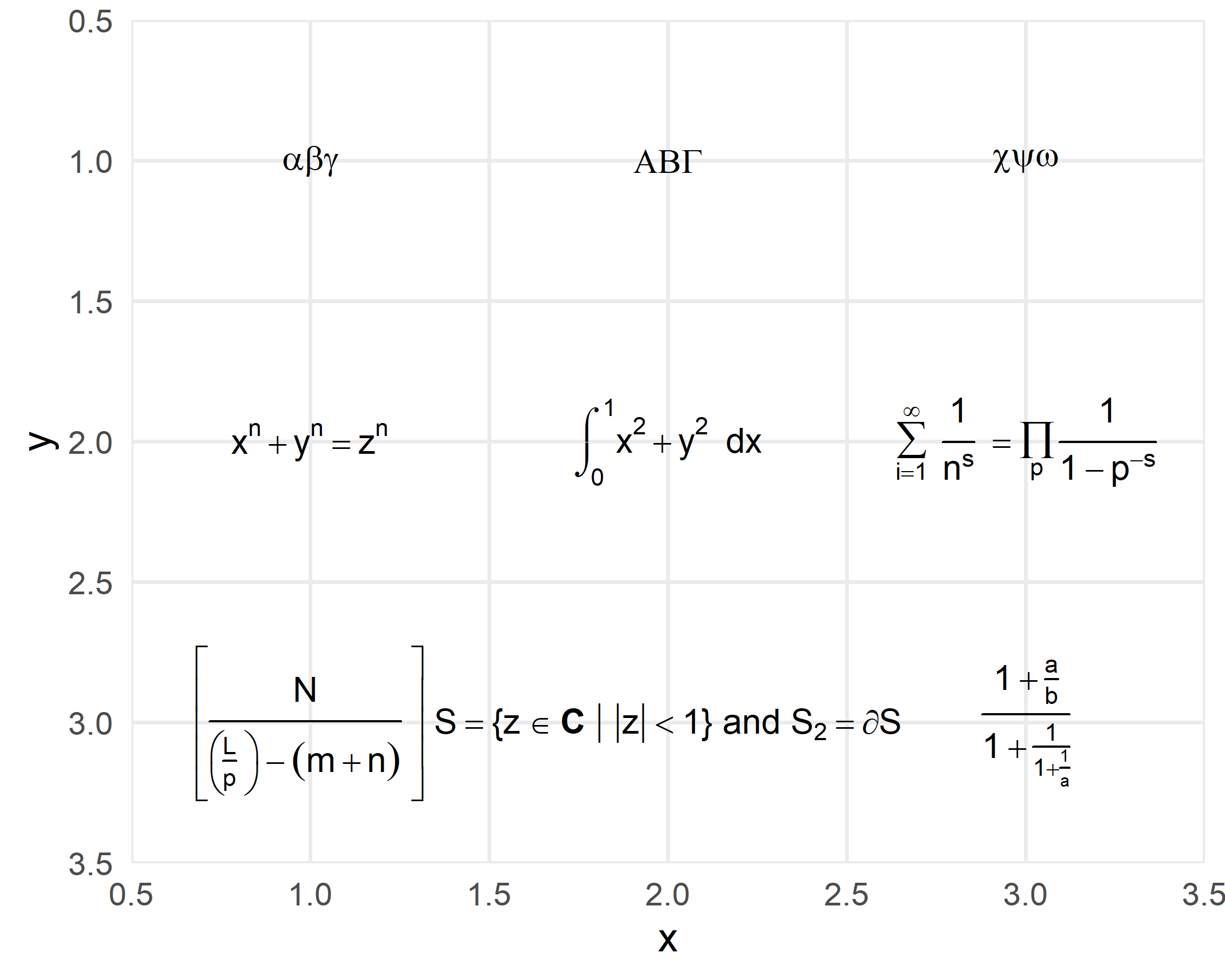
ggplot(df) +
  geom_text(
    aes(
      x = x, y = y, 
      label = TeX(z, output = "character")
    ), 
    parse = TRUE,
    size = 12/.pt
  ) +
  scale_x_continuous(expand = c(0.25, 0)) +
  scale_y_reverse(expand = c(0.25, 0))

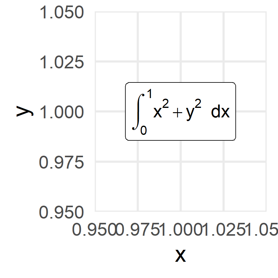
Annotation layers with text or label geoms works exactly the same way.

ggplot() +
  annotate(
    "label", 
    x = 1, y = 1, label = TeX(df$z[5], output = "character"), 
    parse = TRUE
  )

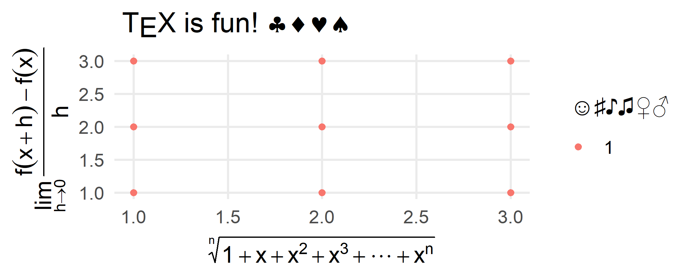
Axis, legend, and plot titles

Axis, legend, and plot titles can be specified directly as expressions, so it isn’t necessary to change the output argument of TeX().

ggplot(df) +
  geom_point(aes(x = x, y = y, color = factor(1))) +
  labs(
    title = TeX(r"( $\TeX$ is fun! $\clubsuit \diamondsuit \heartsuit \spadesuit$ )"),
    x = TeX(r"( $\sqrt[n]{1+x+x^2+x^3+ ... +x^n}$ )"),
    y = TeX(r"( $\lim_{h \rightarrow 0 } \frac{f(x+h)-f(x)}{h}$ )"),
    color = TeX(r"( $\smiley \sharp \eighthnote \twonotes \venus \mars$ )")
  ) 

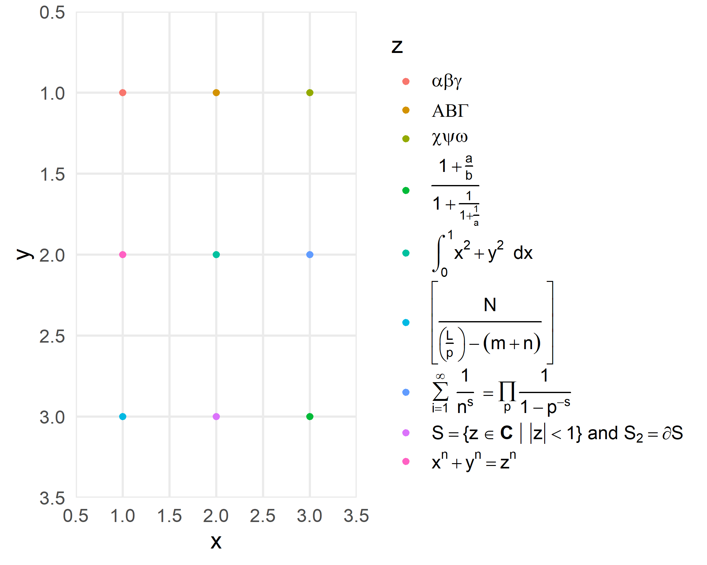
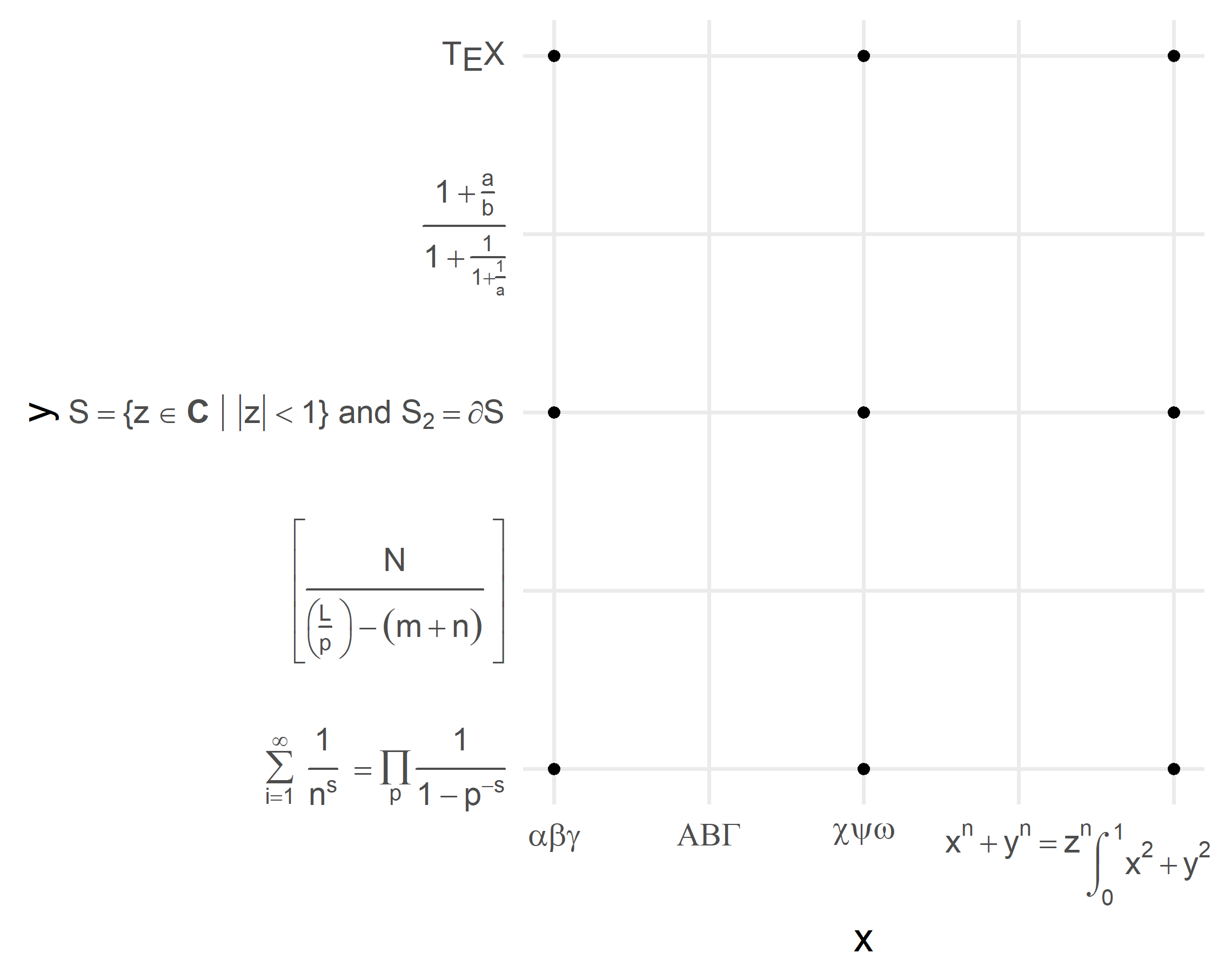
Legend and axis text

In order for the legend and axis text to be displayed correctly, we must use the labels argument of the corresponding scale_*() function.

ggplot(df) +
  geom_point(aes(x = x, y = y, color = z)) + #<<
  scale_color_discrete(labels = TeX(df$z)) + #<<
  scale_x_continuous(expand = c(0.25, 0)) +
  scale_y_reverse(expand = c(0.25, 0)) +
  theme(legend.text.align = 0)

ggplot(df) +
  geom_point(aes(x = x, y = y)) +
  scale_x_continuous(breaks = seq(1, 3, 0.5), labels = TeX(df$z[1:5])) +
  scale_y_continuous(breaks = seq(1, 3, 0.5), 
                     labels = TeX(c(df$z[6:9], r"($\TeX$)"))) 

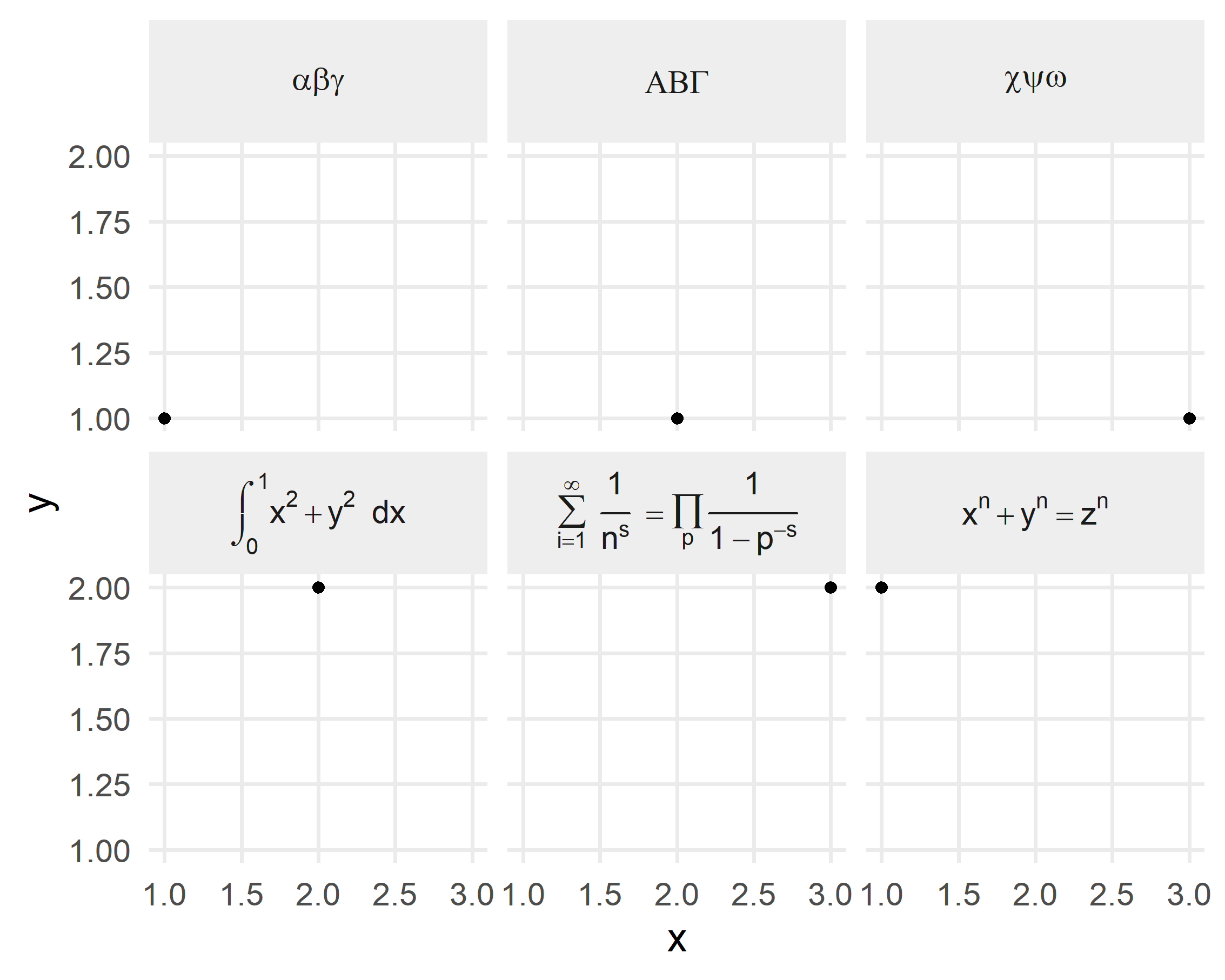
Facet text

To make strip titles work with TeX(), we set the output argument to output = "character". While this is similar to geom_text(), facet_wrap() and facet_grid() have no parse argument to let ggplot2 know that it should interpret the strings as plotmath expressions. Here the trick is to set the label_parsed function as value for the labeller argument.

ggplot(df %>% slice(1:6)) +
  geom_point(aes(x = x, y = y)) +
  facet_wrap(~ TeX(z, output = "character"), labeller = label_parsed)

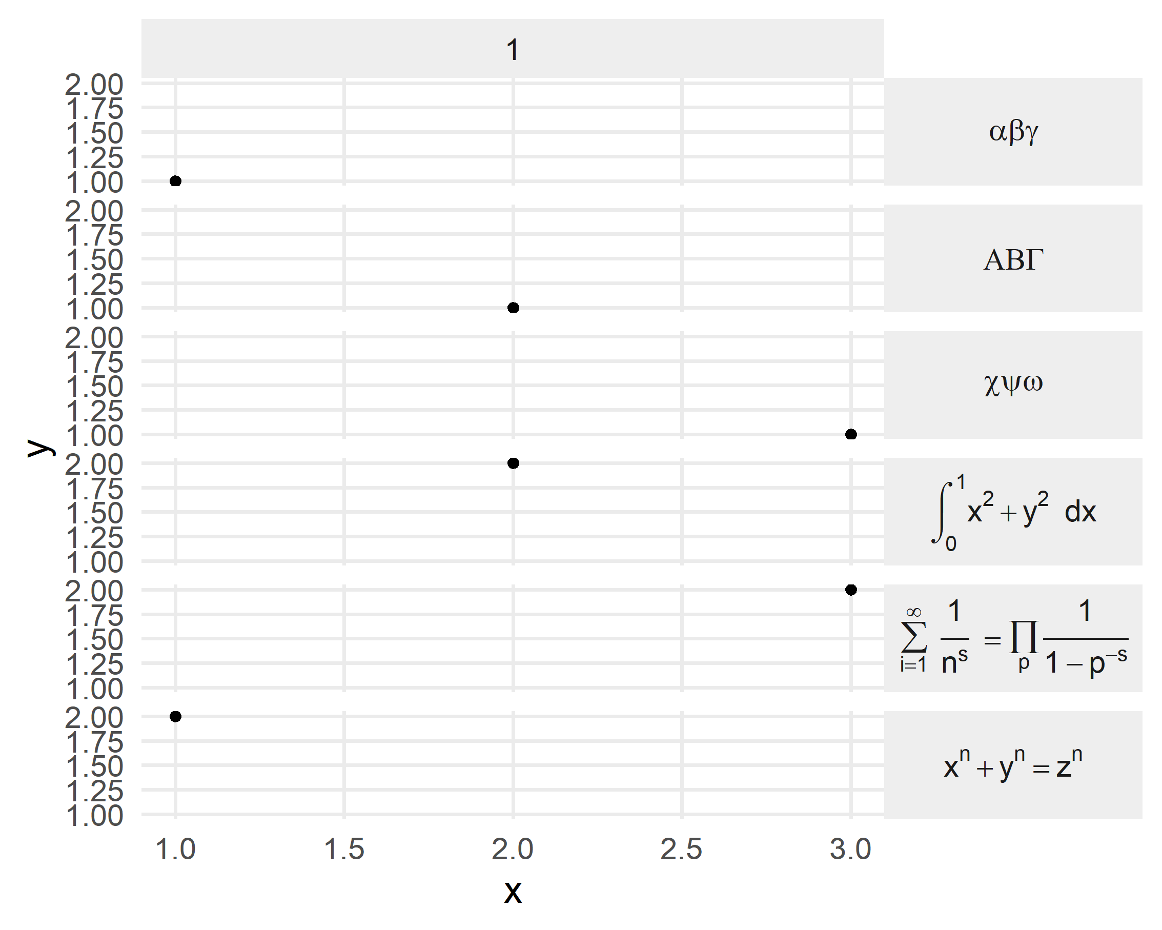
ggplot(df %>% slice(1:6)) +
  geom_point(aes(x = x, y = y)) +
  facet_grid(TeX(z, output = "character") ~ factor(1), 
             labeller = labeller(.rows = label_parsed, .cols = label_value)) +
  theme(strip.text.y = element_text(angle = 0))

Bonus: custom expressions

Almost all expressions of plotmath have an equivalent in latex2exp. Even for the few that are not covered, this isn’t necessarily a problem. Since version 0.9.0 it is possible to create our own LaTeX commands. For example, plotmath’s sup (supremum) and inf (infimum) expressions can be pulled over the user_defined argument of TeX(), see the documentation for details.

plot(
  TeX(r"( $\sup{S}$ )", user_defined = list(r"(\sup)" = r"(sup($arg1))")
)

sessionInfo()

## R Under development (unstable) (2022-02-18 r81760 ucrt)
## Platform: x86_64-w64-mingw32/x64 (64-bit)
## Running under: Windows 10 x64 (build 22000)
## 
## Matrix products: default
## 
## locale:
## [1] LC_COLLATE=German_Germany.utf8  LC_CTYPE=German_Germany.utf8   
## [3] LC_MONETARY=German_Germany.utf8 LC_NUMERIC=C                   
## [5] LC_TIME=German_Germany.utf8    
## 
## attached base packages:
## [1] stats     graphics  grDevices utils     datasets  methods   base     
## 
## other attached packages:
## [1] latex2exp_0.9.3 ggplot2_3.3.5   dplyr_1.0.8    
## 
## loaded via a namespace (and not attached):
##  [1] Rcpp_1.0.8       bslib_0.3.1      compiler_4.2.0   pillar_1.7.0    
##  [5] later_1.3.0      jquerylib_0.1.4  highr_0.9        remotes_2.4.2   
##  [9] tools_4.2.0      digest_0.6.29    gtable_0.3.0     jsonlite_1.7.3  
## [13] evaluate_0.15    lifecycle_1.0.1  tibble_3.1.6     pkgconfig_2.0.3 
## [17] rlang_1.0.1      DBI_1.1.2        cli_3.2.0        rstudioapi_0.13 
## [21] yaml_2.3.4       blogdown_1.8.1   xfun_0.29        fastmap_1.1.0   
## [25] withr_2.4.3      stringr_1.4.0    knitr_1.37       generics_0.1.2  
## [29] fs_1.5.2         sass_0.4.0       vctrs_0.3.8      grid_4.2.0      
## [33] tidyselect_1.1.1 glue_1.6.1       R6_2.5.1         fansi_1.0.2     
## [37] rmarkdown_2.11   farver_2.1.0     purrr_0.3.4      magrittr_2.0.2  
## [41] servr_0.24       codetools_0.2-18 scales_1.1.1     promises_1.2.0.1
## [45] htmltools_0.5.2  ellipsis_0.3.2   usethis_2.1.5    assertthat_0.2.1
## [49] colorspace_2.0-2 httpuv_1.6.5     labeling_0.4.2   utf8_1.2.2      
## [53] stringi_1.7.6    munsell_0.5.0    crayon_1.5.0